Data Analyst Interview Questions 2026: The Complete SQL, Python & Case Study Guide
This data analyst interview questions 2026 guide walks through all five phases with real code.
The 2026 data analyst interview has moved past syntax memorization. Proctored online assessments now evaluate deterministic correctness through tie-breaking, NULL logic, and timeouts; live rounds assess your ability to audit AI-generated code instead of solely writing your own, and product/behavioral rounds focus on judgment rather than recall. This guide covers all five stages of the funnel, 30 fully worked SQL, Python, modern-stack, product-sense, and behavioral questions with real schemas and code, company-by-company benchmarks, and a 14-day study plan.
Part I: The 2026 Interview Landscape & Pre-Screening Strategy
The Two-Stage Technical Funnel
Most 2026 data analyst pipelines run through five distinct phases, and each one tests something different:
- Proctored Online Assessment (OA) — automated grading against a hidden dataset, scored on exact output match.
- Live Machine Coding (SQL) — a human watches you write and debug a query in real time, often on an unfamiliar schema.
- Modern Stack & AI Auditing — can you read someone else’s (or an AI’s) query and find what’s wrong with it on a cloud warehouse?
- Product Case & Experimentation — an open-ended business problem with no single correct query.
- Behavioral & Culture Fit — STAR-format questions about how you’ve actually worked, not how you’d like to be seen working.
Surviving the Automated Proctored Test (OA)
The anti-cheat survival checklist:
- Hardware setup: a single monitor, webcam centered and unobstructed, room well-lit with no other screens visible in the frame.
- Gaze calibration: most platforms flag repeated looking away from the screen — read the full question on-screen rather than on a second device, even a phone in your lap.
- Browser integrity: close every other tab and application before starting; tab-switch detection is standard, and a single flagged switch can end the session.
- Touchpad gestures: disable multi-finger swipe gestures that might trigger an accidental screen or window switch — this trips more candidates than actual cheating does.
The seven hidden grader traps. Automated graders compare your output to a hidden expected result, examining both the row and column types — these are the seven ways a technically “correct” query can still fail:
- Non-deterministic
ORDER BY— an unordered result with tied values can return in a different row order than the grader expects. Always resolve ties using a clear multi-columnORDER BY. - Three-valued logic (
NOT INvs.NULL) —NOT IN (subquery)silently returns zero rows if that subquery contains even one NULL. UseNOT EXISTSor aLEFT JOIN ... WHERE ... IS NULLpattern instead. - Date gaps in moving averages (
ROWSvs.RANGE) —ROWS BETWEENcounts physical rows;RANGE BETWEENcounts logical date values. They diverge the moment your timestamps have a gap, and most 7-day trailing average bugs come from picking the wrong one. - Integer division truncation —
5 / 2silently returns2instead of2.5on many engines unless you explicitly cast to a decimal type. - Dialect-specific syntax crashes — a query written and tested in PostgreSQL (
FILTER,::casts) can fail outright on MySQL or SQL Server. Know which engine the platform runs before you lean on shortcuts. - Statement timeouts (Cartesian join limits) — a missing or wrong join condition on two large tables produces a Cartesian product that blows the grader’s execution time limit and returns a timeout, not a wrong-answer verdict, which is easy to misdiagnose mid-test.
- The
CURRENT_DATEstatic dataset trap — this is the one most candidates never see coming. OA platforms grade against a dataset frozen at a specific snapshot time, but the grading server’s system clock keeps moving forward. If you calculate “days since last order” usingCURRENT_DATEorNOW(), your result silently drifts further from the expected answer every day the question stays live, because the data is frozen but the clock isn’t. The fix is to anchor “today” toMAX(order_date)(orMAX(event_timestamp)) from the dataset itself, rather than using the system clock, unless the question explicitly states that the platform simulates the system date to match the data.
Want to practice these patterns hands-on before your interview? Every schema and query pattern in Parts II and III below is the kind of thing you can drill against real data — browse the BloomInData Dataset Library for practice datasets you can load into your own SQL sandbox or pandas notebook and rebuild these exact queries yourself.
Part II: SQL Technical Questions (OA & Live Deep-Dive)
The SQL section of this data analyst interview questions 2026 guide covers the ten patterns that come up most often across OAs and live rounds. Every question below includes the full DDL schema, sample input rows, the expected output, and the production query.
Core Joins & Aggregations
Q1: High-Velocity Customer Segmentation
CREATE TABLE customers (
    customer_id INT PRIMARY KEY,
    signup_date DATE
);

CREATE TABLE orders (
    order_id INT PRIMARY KEY,
    customer_id INT,
    order_date DATE,
    order_amount DECIMAL(10,2)
);
Sample customers:
| customer_id | signup_date |
|---|---|
| 101 | 2026-01-05 |
| 102 | 2026-02-10 |
| 103 | 2026-01-20 |
Sample orders:
| order_id | customer_id | order_date | order_amount |
|---|---|---|---|
| 1 | 101 | 2026-08-01 | 1200 |
| 2 | 101 | 2026-08-15 | 800 |
| 3 | 101 | 2026-08-28 | 950 |
| 4 | 102 | 2026-08-10 | 500 |
| 5 | 103 | 2026-08-05 | 2200 |
Task: find customers who placed 3+ orders in the last 30 days from the most recent order date in the table.
SELECT
    c.customer_id,
    COUNT(o.order_id) AS orders_last_30d
FROM customers c
JOIN orders o ON o.customer_id = c.customer_id
WHERE o.order_date >= (SELECT MAX(order_date) FROM orders) - INTERVAL '30 days'
GROUP BY c.customer_id
HAVING COUNT(o.order_id) >= 3;
Expected output:
| customer_id | orders_last_30d |
|---|---|
| 101 | 3 |
The trap here is using CURRENT_DATE instead of anchoring to the dataset’s own max date — see hidden trap #7 above.
Q2: Net Realized GMV by Category
CREATE TABLE order_items (
    order_item_id INT PRIMARY KEY,
    order_id INT,
    category VARCHAR(50),
    gross_amount DECIMAL(10,2),
    refund_amount DECIMAL(10,2)
);
Sample data:
| order_item_id | order_id | category | gross_amount | refund_amount |
|---|---|---|---|---|
| 1 | 1 | Electronics | 5000 | NULL |
| 2 | 1 | Apparel | 1200 | 1200 |
| 3 | 2 | Electronics | 3000 | 500 |
| 4 | 3 | Grocery | 800 | NULL |
Task: net realized GMV (gross minus refunds, treating missing refund data as zero, not excluding the row) per category.
SELECT
    category,
    SUM(gross_amount) AS gross_gmv,
    SUM(COALESCE(refund_amount, 0)) AS total_refunds,
    SUM(gross_amount - COALESCE(refund_amount, 0)) AS net_gmv
FROM order_items
GROUP BY category
ORDER BY net_gmv DESC;
Expected output:
| category | gross_gmv | total_refunds | net_gmv |
|---|---|---|---|
| Electronics | 8000 | 500 | 7500 |
| Grocery | 800 | 0 | 800 |
| Apparel | 1200 | 1200 | 0 |
The bug most candidates ship: gross_amount - refund_amount without COALESCE silently turns any row with a NULL refund into a NULL net value, which then vanishes from a naive SUM.
Q3: Customer Retention Anti-Join
CREATE TABLE customers (
    customer_id INT PRIMARY KEY
);

CREATE TABLE orders_2026 (
    order_id INT PRIMARY KEY,
    customer_id INT,
    order_date DATE
);
Sample customers: 101, 102, 103, 104
Sample orders_2026:
| order_id | customer_id | order_date |
|---|---|---|
| 1 | 101 | 2026-03-01 |
| 2 | 103 | 2026-06-01 |
Task: find customers with zero orders in 2026, safely — without a NOT IN NULL trap.
SELECT c.customer_id
FROM customers c
LEFT JOIN orders_2026 o ON o.customer_id = c.customer_id
WHERE o.customer_id IS NULL;
Expected output:
| customer_id |
|---|
| 102 |
| 104 |
If orders_2026.customer_id can contain a NULL row for any reason, customer_id NOT IN (SELECT customer_id FROM orders_2026) returns an empty set entirely — this LEFT JOIN ... IS NULL pattern (or NOT EXISTS) is immune to that.
Advanced Window Functions
Q4: Department Salary Ranking
CREATE TABLE employees (
    employee_id INT PRIMARY KEY,
    department VARCHAR(50),
    salary DECIMAL(10,2)
);
Sample data:
| employee_id | department | salary |
|---|---|---|
| 1 | Analytics | 120000 |
| 2 | Analytics | 120000 |
| 3 | Analytics | 95000 |
| 4 | Engineering | 150000 |
SELECT
    employee_id,
    department,
    salary,
    DENSE_RANK() OVER (PARTITION BY department ORDER BY salary DESC) AS salary_rank
FROM employees;
Expected output:
| employee_id | department | salary | salary_rank |
|---|---|---|---|
| 1 | Analytics | 120000 | 1 |
| 2 | Analytics | 120000 | 1 |
| 3 | Analytics | 95000 | 2 |
| 4 | Engineering | 150000 | 1 |
DENSE_RANK gives tied salaries the same rank with no gap in the sequence that follows — RANK would have skipped straight to 3 for employee 3, which is usually not what “top 2 earners per department” actually means.
Q7: 7-Day Trailing Moving Average
CREATE TABLE daily_revenue (
    revenue_date DATE PRIMARY KEY,
    revenue DECIMAL(10,2)
);
Sample data (7 consecutive days, no gaps):
| revenue_date | revenue |
|---|---|
| 2026-09-01 | 1000 |
| 2026-09-02 | 1200 |
| 2026-09-03 | 900 |
| 2026-09-04 | 1500 |
| 2026-09-05 | 1100 |
| 2026-09-06 | 1300 |
| 2026-09-07 | 1400 |
SELECT
    revenue_date,
    revenue,
    AVG(revenue) OVER (
        ORDER BY revenue_date
        ROWS BETWEEN 6 PRECEDING AND CURRENT ROW
    ) AS trailing_7d_avg
FROM daily_revenue
ORDER BY revenue_date;
Expected output (last row shown):
| revenue_date | revenue | trailing_7d_avg |
|---|---|---|
| 2026-09-07 | 1400 | 1200.0 |
ROWS BETWEEN counts the 6 preceding rows regardless of date gaps. If a day is missing from the table entirely, ROWS still averages the 6 nearest rows present, silently including data from further back in time than 7 calendar days — for a true calendar-day window with gaps, RANGE BETWEEN INTERVAL '6 days' PRECEDING AND CURRENT ROW is the correct choice instead.
Q8: Pareto 80/20 Revenue Contribution Share
CREATE TABLE product_revenue (
    product_id INT PRIMARY KEY,
    revenue DECIMAL(10,2)
);
Sample data:
| product_id | revenue |
|---|---|
| 1 | 5000 |
| 2 | 3000 |
| 3 | 1500 |
| 4 | 500 |
SELECT
    product_id,
    revenue,
    ROUND(
        100.0 * SUM(revenue) OVER (ORDER BY revenue DESC ROWS UNBOUNDED PRECEDING)
        / SUM(revenue) OVER (), 1
    ) AS cumulative_pct
FROM product_revenue
ORDER BY revenue DESC;
Expected output:
| product_id | revenue | cumulative_pct |
|---|---|---|
| 1 | 5000 | 50.0 |
| 2 | 3000 | 80.0 |
| 3 | 1500 | 95.0 |
| 4 | 500 | 100.0 |
The second window function, SUM(revenue) OVER () with no ORDER BY or frame, is deliberately unpartitioned and unordered — it just computes the grand total against every row, which is what makes the percentage denominator constant while the numerator accumulates.
Complex Time-Series & Architecture
Q5: Calendar-Aware Month-over-Month Growth
CREATE TABLE monthly_revenue (
    revenue_month DATE,
    revenue DECIMAL(10,2)
);
Sample data (note: March is missing — a real gap):
| revenue_month | revenue |
|---|---|
| 2026-01-01 | 10000 |
| 2026-02-01 | 12000 |
| 2026-04-01 | 9000 |
WITH calendar AS (
    SELECT generate_series(
        (SELECT MIN(revenue_month) FROM monthly_revenue),
        (SELECT MAX(revenue_month) FROM monthly_revenue),
        INTERVAL '1 month'
    )::DATE AS revenue_month
),
filled AS (
    SELECT
        c.revenue_month,
        COALESCE(m.revenue, 0) AS revenue
    FROM calendar c
    LEFT JOIN monthly_revenue m ON m.revenue_month = c.revenue_month
)
SELECT
    revenue_month,
    revenue,
    revenue - LAG(revenue) OVER (ORDER BY revenue_month) AS mom_change
FROM filled
ORDER BY revenue_month;
Expected output:
| revenue_month | revenue | mom_change |
|---|---|---|
| 2026-01-01 | 10000 | NULL |
| 2026-02-01 | 12000 | 2000 |
| 2026-03-01 | 0 | -12000 |
| 2026-04-01 | 9000 | 9000 |
Without the generate_series calendar spine, LAG() would silently compare April directly against February, reporting a -3000 change and hiding the fact that March had zero recorded revenue entirely. generate_series is PostgreSQL-specific — on Snowflake, use a recursive CTE or a date-dimension table; on BigQuery, GENERATE_DATE_ARRAY.
Q6: User Session Streaks (Gaps-and-Islands)
CREATE TABLE login_events (
    user_id INT,
    login_date DATE
);
Sample data for one user:
| user_id | login_date |
|---|---|
| 1 | 2026-09-01 |
| 1 | 2026-09-02 |
| 1 | 2026-09-03 |
| 1 | 2026-09-06 |
| 1 | 2026-09-07 |
WITH numbered AS (
    SELECT
        user_id,
        login_date,
        ROW_NUMBER() OVER (PARTITION BY user_id ORDER BY login_date) AS rn
    FROM login_events
),
islands AS (
    SELECT
        user_id,
        login_date,
        login_date - (rn * INTERVAL '1 day') AS island_id
    FROM numbered
)
SELECT
    user_id,
    island_id,
    MIN(login_date) AS streak_start,
    MAX(login_date) AS streak_end,
    COUNT(*) AS streak_length
FROM islands
GROUP BY user_id, island_id
ORDER BY streak_start;
Expected output:
| user_id | streak_start | streak_end | streak_length |
|---|---|---|---|
| 1 | 2026-09-01 | 2026-09-03 | 3 |
| 1 | 2026-09-06 | 2026-09-07 | 2 |
Subtracting a running row number (as an interval) from each date collapses every consecutive run of dates onto the same constant island_id value — this is the standard gaps-and-islands pattern and shows up constantly in streak, session, and subscription-continuity questions.
Q9: Rolling 30-Day Churn Identification
CREATE TABLE orders (
    order_id INT PRIMARY KEY,
    customer_id INT,
    order_date DATE
);
Sample data:
| order_id | customer_id | order_date |
|---|---|---|
| 1 | 201 | 2026-07-01 |
| 2 | 201 | 2026-07-20 |
| 3 | 202 | 2026-08-25 |
| 4 | 203 | 2026-05-01 |
WITH last_order AS (
    SELECT
        customer_id,
        MAX(order_date) AS last_order_date
    FROM orders
    GROUP BY customer_id
)
SELECT
    customer_id,
    last_order_date,
    (SELECT MAX(order_date) FROM orders) - last_order_date AS days_since_last_order,
    CASE
        WHEN (SELECT MAX(order_date) FROM orders) - last_order_date > 30
        THEN 'Churned'
        ELSE 'Active'
    END AS churn_status
FROM last_order;
Expected output (assuming dataset max date is 2026-08-25):
| customer_id | last_order_date | days_since_last_order | churn_status |
|---|---|---|---|
| 201 | 2026-07-20 | 36 | Churned |
| 202 | 2026-08-25 | 0 | Active |
| 203 | 2026-05-01 | 116 | Churned |
Same anchoring principle as Q1 and hidden trap #7 — “today” is derived from the data, never the live system clock.
Q10: Multi-Month User Cohort Retention Matrix
CREATE TABLE customers (
    customer_id INT PRIMARY KEY,
    signup_month DATE
);

CREATE TABLE orders (
    order_id INT PRIMARY KEY,
    customer_id INT,
    order_date DATE
);
Sample customers:
| customer_id | signup_month |
|---|---|
| 1 | 2026-06-01 |
| 2 | 2026-06-01 |
| 3 | 2026-07-01 |
Sample orders:
| order_id | customer_id | order_date |
|---|---|---|
| 1 | 1 | 2026-06-15 |
| 2 | 1 | 2026-07-10 |
| 3 | 2 | 2026-06-20 |
| 4 | 3 | 2026-07-05 |
| 5 | 3 | 2026-08-12 |
WITH activity AS (
    SELECT DISTINCT
        c.customer_id,
        c.signup_month AS cohort_month,
        DATE_TRUNC('month', o.order_date) AS active_month
    FROM customers c
    JOIN orders o ON o.customer_id = c.customer_id
)
SELECT
    cohort_month,
    active_month,
    (EXTRACT(YEAR FROM active_month) - EXTRACT(YEAR FROM cohort_month)) * 12 +
    (EXTRACT(MONTH FROM active_month) - EXTRACT(MONTH FROM cohort_month)) AS month_number,
    COUNT(DISTINCT customer_id) AS retained_customers
FROM activity
GROUP BY cohort_month, active_month
ORDER BY cohort_month, month_number;
Expected output:
| cohort_month | active_month | month_number | retained_customers |
|---|---|---|---|
| 2026-06-01 | 2026-06-01 | 0 | 2 |
| 2026-06-01 | 2026-07-01 | 1 | 1 |
| 2026-07-01 | 2026-07-01 | 0 | 1 |
| 2026-07-01 | 2026-08-01 | 1 | 1 |
month_number (months since acquisition) is what actually lets you pivot this into a standard cohort retention matrix in Excel or a BI tool afterward — a raw calendar-month label alone can’t be compared across cohorts with different start dates.
Part III: Python & Pandas Machine Coding
These data analyst interview questions 2026 Python questions mirror the same patterns tested in the SQL section, just in pandas. Each question includes the sample DataFrame structure and the actual printed output.
Q11: Time-Aware Moving Average on Irregular Data
import pandas as pd

df = pd.DataFrame({
    'event_time': pd.to_datetime([
        '2026-09-01 09:00', '2026-09-01 09:05', '2026-09-01 09:40',
        '2026-09-01 10:00', '2026-09-01 10:03'
    ]),
    'value': [10, 12, 30, 15, 14]
})
print(df)
event_time value
0 2026-09-01 09:00:00 10
1 2026-09-01 09:05:00 12
2 2026-09-01 09:40:00 30
3 2026-09-01 10:00:00 15
4 2026-09-01 10:03:00 14df = df.set_index('event_time')
df['rolling_30min_avg'] = df['value'].rolling('30min').mean()
print(df) value rolling_30min_avg
event_time
2026-09-01 09:00:00 10 10.0
2026-09-01 09:05:00 12 11.0
2026-09-01 09:40:00 30 30.0
2026-09-01 10:00:00 15 22.5
2026-09-01 10:03:00 14 14.5A standard integer-position .rolling(3) would average 3 rows, ignoring that the gap between rows 1 and 2 is 35 minutes while the gap between rows 3 and 4 is only 3 minutes. .rolling('30min') on a DatetimeIndex correctly uses only the rows that actually fall inside the trailing 30-minute time window, whatever their count.
Q12: Outlier Trimming via Interquartile Range
df = pd.DataFrame({
    'employee_id': range(1, 9),
    'monthly_salary': [45000, 47000, 46000, 48000, 44000, 46500, 250000, 45500]
})
print(df)
employee_id monthly_salary
0 1 45000
1 2 47000
2 3 46000
3 4 48000
4 5 44000
5 6 46500
6 7 250000
7 8 45500q1 = df['monthly_salary'].quantile(0.25)
q3 = df['monthly_salary'].quantile(0.75)
iqr = q3 - q1
lower_bound = q1 - 1.5 * iqr
upper_bound = q3 + 1.5 * iqr
clean_df = df[(df['monthly_salary'] >= lower_bound) & (df['monthly_salary'] <= upper_bound)]
print(clean_df) employee_id monthly_salary
0 1 45000
1 2 47000
2 3 46000
3 4 48000
4 5 44000
5 6 46500
7 8 45500mean ± 2*std fails here specifically because the one extreme outlier (250000) inflates both the mean and the standard deviation used to detect it — the very value distorting the measurement is used to measure itself. The IQR method is robust because the 25th/75th percentiles barely move when one value in eight is extreme.
Q13: Merging Dirty Datasets with Audit Flags
orders = pd.DataFrame({
    'order_id': [1, 2, 3, 4],
    'customer_id': [101, 102, 103, 999]
})
customers = pd.DataFrame({
    'customer_id': [101, 102, 103],
    'customer_name': ['Asha', 'Ravi', 'Meena']
})
print(orders)
print(customers)
order_id customer_id
0 1 101
1 2 102
2 3 103
3 4 999
customer_id customer_name
0 101 Asha
1 102 Ravi
2 103 Meenamerged = orders.merge(customers, on='customer_id', how='left', indicator=True)
orphans = merged[merged['_merge'] == 'left_only']
print(merged)
print(orphans) order_id customer_id customer_name _merge
0 1 101 Asha both
1 2 102 Ravi both
2 3 103 Meena both
3 4 999 NaN left_only
order_id customer_id customer_name _merge
3 4 999 NaN left_onlyindicator=True adds a _merge column flagging exactly which rows matched, which rows exist only in the left table, and which exist only in the right — without it, order 4’s broken foreign key (customer_id 999, which doesn’t exist in customers) would just silently produce a NaN row that’s easy to miss in a larger dataset.
Q14: Multi-Index Pivot Tables with Cohort Imputation
df = pd.DataFrame({
    'cohort_month': ['2026-06', '2026-06', '2026-07', '2026-07', '2026-07'],
    'active_month': ['2026-06', '2026-07', '2026-07', '2026-08', '2026-09'],
    'region': ['North', 'North', 'South', 'South', 'South'],
    'active_users': [100, 60, 80, 50, 20]
})
print(df)
cohort_month active_month region active_users
0 2026-06 2026-06 North 100
1 2026-06 2026-07 North 60
2 2026-07 2026-07 South 80
3 2026-07 2026-08 South 50
4 2026-07 2026-09 South 20pivot = pd.pivot_table(
df,
index=['region', 'cohort_month'],
columns='active_month',
values='active_users',
aggfunc='sum',
fill_value=0
)
print(pivot)active_month 2026-06 2026-07 2026-08 2026-09
region cohort_month
North 2026-06 100 60 0 0
South 2026-07 0 80 50 20fill_value=0 is what converts a naturally sparse cohort matrix (most region/cohort/month combinations simply never occurred) into a clean, presentable grid instead of one riddled with NaN — the equivalent of pd.Grouper matters when active_month needs to be resampled to a fixed monthly frequency rather than read as whatever string labels happened to appear in the raw data.
Q15: Vectorized Conversion Funnel
df = pd.DataFrame({
    'campaign': ['A', 'B', 'C', 'D'],
    'visitors': [1000, 500, 0, 200],
    'conversions': [50, 25, 0, 10]
})
print(df)
campaign visitors conversions
0 A 1000 50
1 B 500 25
2 C 0 0
3 D 200 10import numpy as np
df['conversion_rate'] = np.where(
df['visitors'] > 0,
df['conversions'] / df['visitors'],
np.nan
)
print(df) campaign visitors conversions conversion_rate
0 A 1000 50 0.05
1 B 500 25 0.05
2 C 0 0 NaN
3 D 200 10 0.05A plain df['conversions'] / df['visitors'] throws a runtime warning and silently produces inf or NaN inconsistently for the zero-visitor row, which can corrupt downstream aggregation. np.where makes the zero-division case an explicit, intentional NaN rather than an accidental one — and it stays fully vectorized, with no slow row-by-row .apply().
Practicing the pandas side too? The BloomInData Dataset Library has messier, real-world datasets worth running these same cleaning and merging patterns against.
Part IV: The Modern Data Stack & Data Modeling
Q16: Auditing AI-Generated SQL
An AI assistant is asked to find “total revenue per customer” and returns:
SELECT c.customer_id, SUM(o.order_amount) AS total_revenue
FROM customers c, orders o
GROUP BY c.customer_id;
What’s wrong with it? There’s no join condition — the comma-separated FROM customers c, orders o is an implicit cross join. Every customer row is paired with every order row regardless of whether they belong together, and SUM then fans out the total revenue by a multiple equal to the customer count. The fix adds the missing predicate: FROM customers c JOIN orders o ON o.customer_id = c.customer_id. This is the single most common AI-generated SQL bug candidates are now expected to catch on sight, because it produces a plausible-looking, badly wrong number rather than an error.
Q17: Snowflake QUALIFY Clause
Task: get each customer’s most recent order without a nested CTE.
SELECT
    customer_id,
    order_id,
    order_date,
    ROW_NUMBER() OVER (PARTITION BY customer_id ORDER BY order_date DESC) AS rn
FROM orders
QUALIFY rn = 1;
QUALIFY filters on a window function’s result the way HAVING filters on an aggregate — without it, you’d need to wrap the ROW_NUMBER() query in an outer SELECT ... WHERE rn = 1, since window functions can’t be referenced in the same WHERE clause that computes them. QUALIFY is Snowflake and BigQuery-supported; it isn’t standard ANSI SQL, so it won’t run on PostgreSQL, MySQL, or SQL Server.
Q18: BigQuery Arrays (Unnesting Semi-Structured JSON)
CREATE TABLE events (
    user_id INT64,
    session_id STRING,
    page_views ARRAY<STRING>
);
Sample row: user_id=1, session_id='s1', page_views=['home', 'product', 'cart', 'checkout']
SELECT
    user_id,
    session_id,
    page AS page_view,
    OFFSET AS view_order
FROM events, UNNEST(page_views) AS page WITH OFFSET;
Expected output:
| user_id | session_id | page_view | view_order |
|---|---|---|---|
| 1 | s1 | home | 0 |
| 1 | s1 | product | 1 |
| 1 | s1 | cart | 2 |
| 1 | s1 | checkout | 3 |
UNNEST explodes an ARRAY column into one row per element, which is the standard way to flatten nested event or clickstream data stored natively in BigQuery before running any per-page-view aggregation.
Q19: Analytics Engineering — dbt Idempotency
A dbt model uses unique_key: order_id in an incremental config:
{{
  config(
    materialized='incremental',
    unique_key='order_id'
  )
}}

SELECT order_id, customer_id, order_amount, updated_at
FROM {{ source('raw', 'orders') }}
{% if is_incremental() %}
WHERE updated_at > (SELECT MAX(updated_at) FROM {{ this }})
{% endif %}
Why does unique_key matter here? Without it, every incremental run would simply append new rows, including updated versions of orders that already exist in the table — a single order edited twice would end up duplicated. unique_key tells dbt to merge/upsert on order_id instead of blindly inserting, which is what makes the model idempotent: running it twice on the same data produces the same table, not a growing pile of duplicates.
Q20: Text-to-SQL Governance
Scenario: a stakeholder pastes an AI-generated SQL query into a dashboard and asks you to validate it before it goes live. What’s your review checklist?
Confirm every join has an explicit, correct condition (no implicit cross joins, per Q16). Confirm date filters anchor to the data’s own max timestamp, not a hardcoded or system date. Check aggregate functions against NULLs — a SUM or AVG silently drops NULL rows rather than erroring, which can understate a metric without any visible failure. Verify the metric definition matches an existing, governed definition elsewhere in the business (two dashboards showing different “active users” numbers from two different AI-written queries is a fast way to lose stakeholder trust). Run the query against a known historical period and reconcile it against a number you can already verify by hand before publishing it anywhere.
BI Tool Logic & Modeling
Q20b: Resolving Many-to-Many Relationships in Star Schemas
Scenario: a students table and a courses table both connect through an enrollments bridge table, and a report needs total enrollment count per course. A direct many-to-many relationship between students and courses confuses most BI tools’ filter propagation — a filter applied on the students side won’t reliably cascade through to courses correctly. The fix is to make enrollments its own fact table with two one-to-many relationships (one from students, one from courses) into it, rather than modeling a direct many-to-many link between the two dimension tables. This is the standard “bridge table” pattern.
Q20c: Tableau Level of Detail (LOD) Calculations for Baseline Metrics
Task: show each customer’s total spend as a % of their own first-month spend, regardless of which month is currently filtered on the dashboard.
// Baseline: each customer's spend in their signup month, fixed regardless of filters
{ FIXED [Customer ID] : SUM(
    IF DATETRUNC('month', [Order Date]) = { FIXED [Customer ID] : MIN(DATETRUNC('month', [Order Date])) }
    THEN [Order Amount] END
) }
A regular calculated field recomputes every time a dashboard filter changes, which breaks a “vs. baseline” comparison the moment someone filters to a specific month — because at that point, there’s no earlier month left in the view to compare against. A FIXED LOD expression computes its result at the specified level of detail (here, per customer) independent of whatever’s currently filtered on the sheet.
Q20d: Power BI DAX Row Context vs. Filter Context (CALCULATE)
Total Sales = SUM(Orders[order_amount])

Sales Same Category =
CALCULATE(
    [Total Sales],
    ALLEXCEPT(Orders, Orders[category])
)
A measure like [Total Sales] inside a table visual evaluates in row context — one row at a time. CALCULATE is what shifts a measure into a new filter context: here, ALLEXCEPT(Orders, Orders[category]) strips every filter currently applied to the Orders table except the category filter, so Sales Same Category always shows the category total regardless of which other slicers (date, region) are active elsewhere on the report. Confusing row context with filter context is the single most common DAX mistake in interviews.
Part V: Product Sense, A/B Testing & Root-Cause Analytics
Diagnostic Frameworks
Q21: The MECE Root-Cause Framework
Scenario: DAU dropped 15% overnight. Walk through your investigation. Split the drop into mutually exclusive, collectively exhaustive branches so nothing is double-counted and nothing is missed: internal (a recent release, a pricing or UX change, an outage) versus external (seasonality, a competitor event, a holiday). Within “internal,” cut by platform (iOS vs. Android), by user segment (new vs. returning), and by region, since a genuine bug usually shows up disproportionately in one slice rather than uniformly everywhere. Only after isolating the affected slice does root cause get diagnosed.
Q24: Defining “Power Users”
Why is “logged in 5+ times a week” a weak definition of a power user? It’s an arbitrary threshold picked without reference to the actual data. The better approach: plot the full distribution of a usage metric (sessions, actions, spend) across all users, and define “power user” by where a genuine break or long tail actually occurs in that distribution, rather than a round number that sounds intuitive but doesn’t correspond to any real behavioral discontinuity.
Q25: SLA & Operations Diagnostics
Quick-commerce scenario: average delivery time has crept from 11 to 16 minutes over two weeks — where do you look first? Decompose delivery time into its component legs (order acceptance, picking/packing, rider assignment, transit) rather than treating it as one number. Cross-reference against dark-store-level and rider-availability data before assuming a single cause — a 5-minute average increase is often 80% explained by a handful of understaffed stores. FinTech scenario: card authorization success rate dropped 4 points — segment by issuing bank, card network, and transaction amount bucket before escalating, since a single bank’s gateway issue can move the blended average.
Experimentation & Statistics
Q22: Sample Ratio Mismatch (SRM)
An A/B test intended as a 50/50 split actually shows 46% control / 54% treatment. Why should you distrust the p-value before even reading it? A significant deviation from the intended split ratio (checked with a chi-square goodness-of-fit test against the expected 50/50) signals that randomization itself is broken. When SRM is present, any observed treatment effect is confounded with whatever caused the imbalance, and the resulting p-value is uninterpretable regardless of how small it is. SRM is checked before looking at the outcome metric, not after.
Q23: Marketplace Network Effects — Why Switchback Testing
Why would a ride-hailing or food-delivery marketplace use switchback testing instead of standard user-level A/B testing for a pricing or matching algorithm change? User-level randomization assumes each unit’s outcome is independent of every other unit’s assignment (SUTVA). In a two-sided marketplace, that assumption breaks: a driver in treatment competing for the same rider pool as a driver in control means the two arms interfere through shared supply. Switchback testing randomizes at the level of a geographic zone and a time window instead, so supply and demand within a period are consistently exposed to the same condition.
Part VI: Behavioral & Stakeholder Communication (STAR Method)
Q26: When Data Contradicts Executive Intuition
Frame the finding as new information that changes the odds of success, not as a rebuttal. “This data suggests X performs better than the plan assumed — here’s what that could unlock” lands very differently from “the plan was wrong.”
Q27: Handling Ambiguous Requirements
Before writing a single query, restate the request as a testable hypothesis and confirm it with the stakeholder: “when you say ‘engaged users,’ do you mean logged in, or performed a core action?”
Q28: Post-Mortem of a Data Pipeline Outage
Structure the answer around four phases: detection (how the failure was first noticed, and how long that took), containment (what stopped the bad data from spreading further), communication (who was told, how fast), and prevention (the actual fix — a data-quality check, a schema-change alert — not just “we fixed the bug”).
Q29: Prioritizing Ad-Hoc Requests vs. Infrastructure Work
Score competing asks on two axes: urgency (does this block a decision this week) and revenue/business impact (what’s at stake if delayed). A high-urgency, low-impact request gets a fast, minimal answer; a low-urgency, high-impact infrastructure fix gets scheduled, not dropped.
Q30: Explaining Statistical Significance to Stakeholders
Translate the abstraction into commercial terms: “we’re 95% confident this change genuinely increases GMV, and the range of likely impact is between ₹X and ₹Y per month” communicates far more than reciting a p-value.
Part VII: Logistics, Benchmarks & Timelines
Company-Specific Interview Breakdowns
Indicative compensation brackets by company category — these are aggregated ranges from public salary-aggregator data, not officially published figures, so treat them as planning ranges rather than guarantees:
| Company | Bracket | Focus Areas | Typical Range (India) |
|---|---|---|---|
| Google, Amazon | Big Tech / FAANG | Heavy SQL + statistics, scale-oriented case studies | ₹20L–₹35L (mid), ₹30L–₹50L (senior); Amazon specifically trends closer to ₹9.6L–₹12.5L across 1–9 yrs per aggregator averages |
| Flipkart, Swiggy, Zomato, Razorpay, Zepto | Product / Unicorn | Fast-paced product case rounds, funnel and growth metrics | ₹6L–₹9L (fresher), ₹12L–₹22L (mid), ₹20L–₹35L (senior) |
| Uber | Global Product Tech | Marketplace/network-effect experimentation (switchback testing), SQL at scale | Broadly comparable to the unicorn bracket for India-based roles |
| Walmart Global Tech, JPMorgan | GCC / Enterprise | Data modeling discipline, governance, SQL correctness over cleverness | ₹5L–₹7.5L (fresher), ₹10L–₹18L (mid), ₹18L–₹30L (senior) |
The 2-Week Structured Preparation Roadmap
| Days | Focus |
|---|---|
| 1–4 | SQL: joins, aggregation, window functions, all 7 hidden grader traps drilled until automatic |
| 5–6 | Python/pandas: cleaning, merging, time-aware rolling windows, vectorized logic |
| 7–8 | Modern stack: one cloud warehouse’s syntax quirks (QUALIFY, arrays), dbt basics, AI-query auditing practice |
| 9–10 | Product sense & experimentation: MECE decomposition drills, SRM and switchback-testing concepts |
| 11–12 | Behavioral: draft and rehearse all five STAR stories out loud, not just in writing |
| 13 | Full mock OA under proctoring conditions, timed |
| 14 | Review mistakes from the mock, light review only — no new material the day before a real interview |
Frequently Asked Questions
How different is the 2026 SQL interview from a few years ago?
The hard part has shifted from writing correct SQL to writing SQL that survives deterministic grading — tie-breaking, NULL logic, and timezone/date anchoring now account for more failed OAs than actual logic errors.
Is it acceptable to mention using AI tools during interview prep?
Yes, and increasingly expected — what interviewers actually screen for is whether you can audit and correct AI-generated code, not whether you avoided using it.
Should I prepare Tableau or Power BI for these interviews?
Prepare the underlying modeling concepts (star schema, fact/dimension, LOD vs. DAX filter context) first — those transfer directly between tools.
How long should I spend on the behavioral round if my technical skills are strong?
At least two full days, rehearsed out loud. A technically excellent candidate with vague, unstructured behavioral answers is a common and avoidable rejection reason.
What are the most important data analyst interview questions 2026 candidates should prepare for?
SQL joins and window functions carry the most weight, followed by the ability to audit AI-generated code and reason through an open-ended product case — this guide’s Parts II through V cover all three in depth.
About the Author
I'm Priyanka Lakra, a data analyst, explorer, and learner passionate about data analytics, forecasting, and hands-on projects. Through BloomInData, I share my learning journey and the projects I build along the way.
That’s the full set of data analyst interview questions 2026 is testing for — bookmark this before your next OA.